ARTÍCULO PRESENTADO EN ECI-invierno-2014 UNIVERSIDAD RICARDO PALMA
Pueden acceder al artículo y a la presentación originales en los siguientes enlaces:
TEXTO DE PRESENTACIÓN DE ARTÍCULO
Texto del Artículo:
Efecto del transporte público sobre la red de transporte de una ciudad en desarrollo
Transit and the performance of the transportation network of a developing city
Manuel J. Martínez1, y Athanassios K. Bladikas2
1 Profesional Independiente, Calle Schrader179, dpto. 202, San Borja, Lima 41, PERU
2 Interdisdisciplinary Program of Transportation, New Jersey Institute of Technology, USA
Abstract
This paper calculates the effect of transit flows over the performance of the urban transportation network of a developing city, the case of Lima-Callao in Peru. DYNASMART, a dynamic traffic assignment model, is used to collect measures of performance for every hour of the typical working day. It was found that, transit flows in common traffic reduces the performance of the transportation network in between 12 to 25 percent. It was also found that a small effect is caused when an additional Bus Rapid Transit project is considered. Secondary and additional performance indicators are examined with similar results. Fuel consumption and pm10 emissions are measured. Average speed is calculated by time of the day and for 4 major road facilities.
Descriptores: transportation, pollution
The transportation problem in a developing city
In the year 2005, the transportation demand of the city of Lima was estimated at 11.5 millions of motorized trips. The 76 percent were made by bus transit, 16 percent by auto, and 8 percent by taxi [1]. The problem of transportation of the developing city of Lima has been usually analysed as the problem of the transit system. Recently, two areas have been studied to improve the transit system of developing cities: 1) the problems of congestion and pollution caused by the deregulation of transit when composed of numerous small vehicles, and 2) the solution of Bus Rapid Transit (BRT) that allocates lanes to busways and that upgrades the fare collection and the coordination of the bus operations. Besides that, a particularity has been developed in the city of Lima by which, deregulated transit means “oversupply” of transit vehicles, that causes congestion over the transportation network, and therefore, the oversupply of transit vehicles had to be removed from the system.
During the 1980s the public transit companies failed to cope with the increasing population of developing cities, when they could not buy the adequate number of buses due to low fares and scarce funding. A great number of private small vehicles appeared to serve the unsatisfied demand [2]. Private operators got better results because they worked with smaller vehicles, lower labor cost, and more flexible bus operations to attend the demand [3]. Thus, when private ownership and deregulation were applied in several developing cities, congestion and pollution appeared as consequences of these policies [4]. The answer to solve the problems of congestion and pollution appeared from two successful experiences; the BRT of Bogota and the public tendering of transit routes of Santiago [5]. However, even though there was an amount of congestion caused by the increase in the number of transit vehicles, there were not measurements of their effect over the performance of the entire transportation network of a developing city. The allocation of road lanes to busways obtained very high levels of capacity and speed in developing cities [6]. But, in the case of very high number of transit vehicles permitted in busways, the result was a chaos that limited the commercial speed of the busway system [7]. Thus, the BRT was projected to upgrade a busway by using centrally coordinated operations of high capacity buses, and automated fare collection and special passenger accesses that permitted a safe increase of speed over the former system [8]. The BRT was regarded as so successful that it was recommended to extend its functions to be a planning institution to regulate the whole urban transportation of a developing city [9]. However, being busways and BRTs the answers to solve the congestion caused by deregulated transit, by allocating lanes to BRTs, there appears the need to measure the effect of such allocation of lanes over the performance of the transportation network of a developing city. The particularity of the city of Lima is that the great quantity of small buses caused that the transit system were diagnosed as oversupplied, which meant that a number of transit vehicles would have to be taken out of the transit service [10]. A busway project for Lima, funded by the World Bank, set the oversupply up to 1,583 transit vehicles to be reallocated elsewhere [11]. Three years later and over a longer route, the oversupply was calculated a much higher figure between 10,000 to 15,000 transit vehicles according to their own figure of 50 percent oversupply that needed to be eliminated from the route [12].
As a summary, the oversupply of transit vehicles has been associated as a major cause of traffic congestion, but there has not been a measurement of the effect of transit flows over the performance of the transportation network of the developing city of Lima. Moreover, in developing cities like Lima, the bus transit serves most of the motorized trips, but it has been said that policies to promote transit created an amount of congestion onto the transportation network. This paper measures such effect of transit flows and the allocation of lanes to BRT, over the performance of the transportation network of the developing City of Lima.
Methodology of dynamic traffic assignment
The software Dynasmart has been designed to assign time-varying traffic demands and to model the corresponding traffic patterns to evaluate network performance. This software met functional requirements set forth by Federal Highway Administration, including the capability to model traffic disruptions and to describe the vehicle performance characteristics. Dynasmart integrates traffic flow models, path processing methodologies, and behavioral rules into a single simulation-assignment framework [13]. Dynasmart is a transportation network planning tool, used for dynamic network analysis to evaluate the performance of the network under changes in the capacity of the network or in the prevalent conditions of the network [14]. Therefore, this tool can be used to evaluate the performance of a transportation network under the effect of transit flows and/or the allocation of lanes to a BRT.
Building of the data
The transportation network used to build the model is similar to the network used in the Master Plan for the city of Lima and Callao [1] as shown in the Figure 1. The capacity of the network has been updated to 2012 and kept fixed for the analysis for the base year 2005 and to the projected year 2025. The network is composed of 446 zones, 14 super-zones, 6542 nodes, and 14977 links. The geographic area reaches 90 km. South-North by 40 km. East-West. The most populated Central City is a triangle of about 15 km. per side between the Port of Callao to the West, the Center to the East, and the modern area Miraflores-San Isidro-Chorrillos to the South, this is also the most intensive area in the use of autos and taxis, and also the best served by bus transit.
Bus flows were processed for the base year 2005, by using the number of vehicles, frequency, and route as approved by the Municipality of Lima for near 600 bus lines during the peak hour. The bus flows were calculated of each link by using the software EMME3. The projected number of transit vehicles for 2025 was multiplied by 1.34 a projection factor from [1]. In the Dynasmart model, the only transit flows considered are those that occur in links of common traffic, and it does not consider those transit flows in busways nor in the existing South-North 26km BRT. Bus flows appear as very high for individual roads; some examples are transit flows equivalent to 5500 PCU at “Plaza Bolognesi” (six lanes per direction), 1800 PCU at “Plaza Dos de Mayo” (seven lanes per direction), 1500 PCU at “Prolongacion Tacna-Rimac” (three lanes per direction), 2500 PCU at “Paseo Colon” (five lanes per direction), 2600 PCU at “Av. Arica” (six lanes per direction), 2000 PCU at “Av. Aviacion” (three lanes per direction) and so on. Thus, some individual links can accommodate quite a number of transit vehicles. But several of the roads are wide, and the measurement of the total effect of transit over the transportation network is needed. Traffic flow models were adapted to Dynasmart by using a simulation exercise in a small network composed of a 4-mile arterial with two unsignalized intersections and similar level of traffic on the conflicting approaches.
Capacity and speed, as well as the alpha factor, were tuned to render capacities and speed similar to data collected in field studies. See the results of the traffic flow models in Table 1 where it is shown the resulting values for the whole arterial with intersections. The field collection of free flow speed and capacity followed the generally accepted methods [15] and [16]. The observations were used to estimate flow-delay functions. Saturation state of roads occurs when density is maximum and speed is minimum, a very important index for Peruvian legislation that empowers local authorities to take action on public transit. The transportation network of Lima can be described as a big network of low capacity and low speed arterials with one South-North highway of nearly 50 km. and another South-North expressway of 11 km. The average vehicle speed for all private vehicle trips is about 21 mph. The Master Plan estimated Origin Destination matrix for the 24-hour demand was for 2005 and 2025 [1]. These matrices were converted to hour by hour matrices by using several factors published in the same reference. These factors were occupancy rates for autos (2.00) and taxis (0.71), percentage of trips made by autos and taxis by trip purposes, number of motorized trips for each of the 24 hours and by 5 trip purposes, modal share by trip purpose, and modal share and number of trips generated by 14 geographic areas. The Master Plan considered a matrix for auto, and another for taxi. In the case of trucks, the permitted hours for trucks matched with the location of origins [1]. Thus, the trips attributable to fuel cargo, agriculture cargo, other market cargo, and ports were assigned. Percentages of distribution of trips were assumed for each permitted schedule where the prohibition took place. Higher proportion was assigned to the first three hours of permission period. The rest of truck trips formed a small proportion of the total, and it was assumed a distribution over the regular hours of the day with preference after 10am. There was a need for a distribution of trips within the hour, by 5 minutes period, which was taken from special traffic counts made in 2007 by the project 194-2005-CONCYTEC-OAJ. Several distributions were calculated, some increasing, others increasing or flat. Also, some distributions estimated included South-North and East-West directions. The value of time for auto and taxi users was taken as 2.6 dollars per hour, from the reference [17].
Simulation plan
The Dynasmart ran for two planning years 2005 and 2025, the base year and the projected year, respectively. On each year, four cases were considered: “no-transit”, “cap-transit”, “lane-transit”, and “cap-brt-transit”. On each case, the model ran for each of the 24 hours, with five minutes of warming up period. Three OD matrices were considered on each simulation: autos, taxis, and trucks. The case “no-transit” is the baseline for the simulation-assignment process and it is the theoretical state where no transit flows use the roads, only autos, taxis, and trucks. The case of “cap-transit” is where the transit flows effect is introduced in the network as a reduction of the capacity of links by the quantity of transit flows. The case of “lane-transit” is when the transit flows effect is introduced in the network as a reduction of one lane on each link where the transit flows amounted for 0.5 the capacity of a lane, or two lanes where the transit flows amounted for 1.5 the capacity of a lane. It was found that more than 2298 links reduced in one lane in 2005 (15% of network) and 3244 links reduced in one or two lanes in 2025 (22% of network) The case “lane-transit” is the maximum possible effect of transit flows. The case “cap-brt-transit” simulates the effect of allocating lanes to a BRT project as additional reduction of capacity over the case “cap-transit”. The example of BRT is taken from the East-West 24-km BRT Project Central Highway which considers the allocation of one lane per direction [18]. All simulations were set to be run in Sequential mode and One-shot best path (input file system.dat). Also, they all were set to choose the Best path but being non-responsive drivers (input file scenario.dat). Additionally, all the 446 zones are used without aggregation, and only one best path is calculated (input file network.dat). It was assumed for Lima a period of cold starts that consist of the first 13 minutes of vehicle trips in mild weather, which are supposed to spend 80 percent more fuel and to discharge more pollutants. The adjustment was calculated by using the following statistical method: take the hour of smaller and the hour of higher number of vehicle trips and calculate linear equations between the number of vehicles, the number of non-cold starts, the length of trips, and the average speed. The linear equations are taken from a sample of 35 observations of all non-cold start trip segments ordered by the size of the non-cold start segment of the trip, all observations taken from data of the output file VehicleTrajectory.dat which gives the trajectory of all the vehicle trips node by node, and the accumulated travel time at each node. The linear equations are calculated such as from each run, given the average speed and length of trip, it is obtained the fuel spent as well as the pollution emitted in the non-cold-start trip segments.
Measures of performance
The primary performance variables are three, the number of vehicle-hours or intermediate input to produce transportation, the number of vehicle-miles or final product transportation, both taken from the output file SummaryStat.dat, and the average vehicle speed (mph) or productivity, which is the quotient of both numbers. The secondary performance variables are two, the user time cost and the user monetary cost. The user time cost is the cost of the time of the users of autos and taxis. It is calculated by multiplying the array of the output file fort.700.dat of density per minute per link, by the array of link length, by the array of number of lanes, matrix 10×1500 per minute each array, and then applying the occupancy rates and the value of time for auto trips. The monetary cost includes the toll revenue (provided in the TollRevenue.dat file), the maintenance cost of vehicles, and the fuel cost. The maintenance cost of vehicles is calculated from the vehicle hours multiplied by the cost per hour per type of vehicle (3c per auto, 4.4c for truck, and 4.2c for taxi taken from the reference [1]). The quantity of fuel is obtained from the array of speed per link per minute from the output file fort.900.dat and from which the quantity of km/minute is obtained, multiplied by the corresponding rate of consumption of fuel per km. given by a scale of eight levels of speed, and then all multiplied by the number of vehicles on each link on each minute of simulation. The additional performance variables are three, the “inefficiency” factor, the OD travel time, and the daily toll revenues. The “inefficiency” factor is the percentage of all vehicle trips that remain in the network after the simulation period ends.
Table 1 Traffic flow models
| Road
Type |
Traffic Flow Model | Resulting Values | |||||
| Speed
mph |
Capacity | α | Speed
mph |
Capacity | |||
| Art. D | 35 | 1850 | 1.27 | 23 | 850 | ||
| Art. E | 40 | 1800 | 1.50 | 25 | 860 | ||
| Col. | 30 | 1700 | 1.37 | 24 | 600 | ||
| Art. F | 35 | 1350 | 1.38 | 22 | 900 | ||
| Art. B | 30 | 1200 | 1.88 | 18 | 500 | ||
| Hway | 60 | 2200 | 2.75 | 38 | 1350 | ||
| Exway | 75 | 2400 | 1.25 | 62 | 1600 | ||
Table 2 Primary performance indicators
| Year/case | no-transit | cap-transit | lane-transit | cap-brt-transit | ||
| 2005
VH (´000) VM (´000) S (mph) |
658
13,728
20.9 |
728 +11% 13,326 -3% 18.3 -12% |
778 +18% 13,025 -5% 16.8 -20% |
739 +12% 13,255 -3% 18.0 -14% |
||
| 2025
VH (´000) VM (´000) S (mph) |
1,631
21,424
13.2 |
1,834 +12% 20,217 -6% 11.1 -16% |
1,970 +21% 19,350 -10% 9.9 -25% |
1,858 +14% 20,123 -6% 10.9 -17% |
||
Table 3 Secondary, additional performance indicators
| Year/case | no-transit | cap-transit | lane-transit | cap-brt-transit | ||
| 2005
time (´000) $ (´000) Ineff. (%) OD (min.) Tolls$ (´000) |
3,235
5,464
0.34
12.6
162.9 |
3,524 +9% 5,517 +1% 0.39 +15% 13.3 +6% 167.2 +3% |
3,585 +11% 5,255 -4% 0.42 +24% 13.1 +3% 173.5 +7% |
3,577 +11% 5,515 +1% 0.40 +18% 13.3 +6% 164.5 +1% |
||
| 2025
time (´000) $ (´000) Ineff. (%) OD (min.) Tolls$ (´000) |
7,475
8,492
0.51
14.8
183.7 |
8,306 +11% 8,801 +4% 0.57 +12% 16.1 +9% 184.3 0% |
8,385 +12% 8,034 -5% 0.62 +22% 15.4 +4% 213.5 +16% |
8,364 +12% 8,814 +4% 0.58 +14% 16.2 +9% 184.7 +1% |
||
Table 4 Fuel consumption & emissions pm10
| Year/case | no-transit | cap-transit | lane-transit | cap-brt-transit | ||
| 2005
E7.8 (kgal.) B5 (kgal.) LPG (kl.) CNG (k-m3) pm10 (kgr.) |
520
567
358
358
4,897 |
528 +2% 569 +0% 364 +2% 363 +2% 4,941 +1% |
500 -4% 542 -4% 344 -4% 344 -4% 4,703 -4% |
527 +1% 570 +1% 363 +1% 363 +1% 4,943 +1% |
||
| 2025
E7.8 (kgal.) B5 (kgal.) LPG (kl.) CNG (k-m3) pm10 (kgr.) |
883
827
537
536
8,645 |
925 +5% 877 +6% 562 +5% 561 +5% 8,765 -2% |
831 -6% 779 -6% 505 -6% 505 -6% 8,185 -5% |
923 +4% 853 +3% 561 +4% 560 +4% 8,780 +2% |
||
|
|
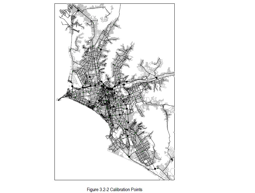
Figure 1.- Transportation Network of Lima-Callao
|
Figure 2.- Reduction in productivity (lower speed) |
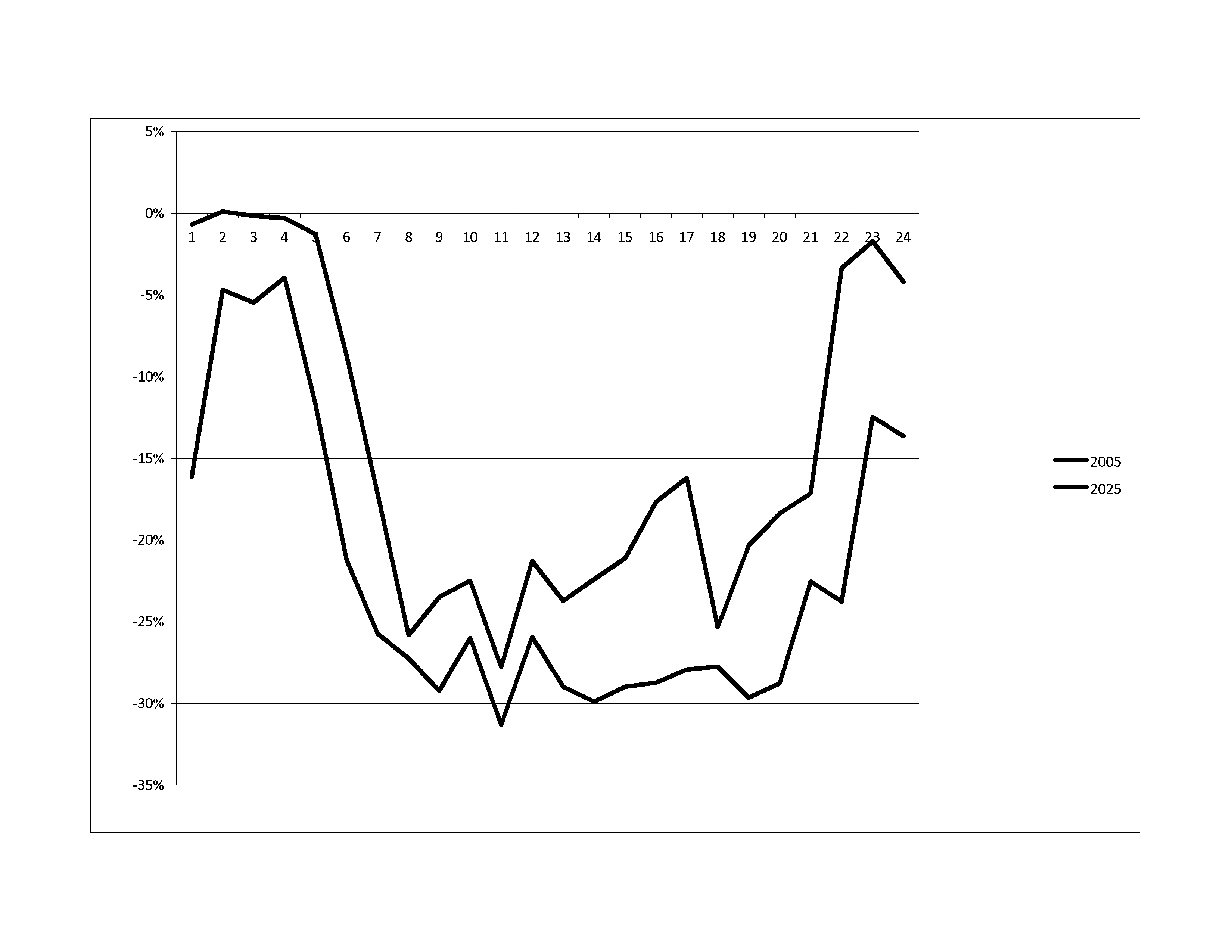
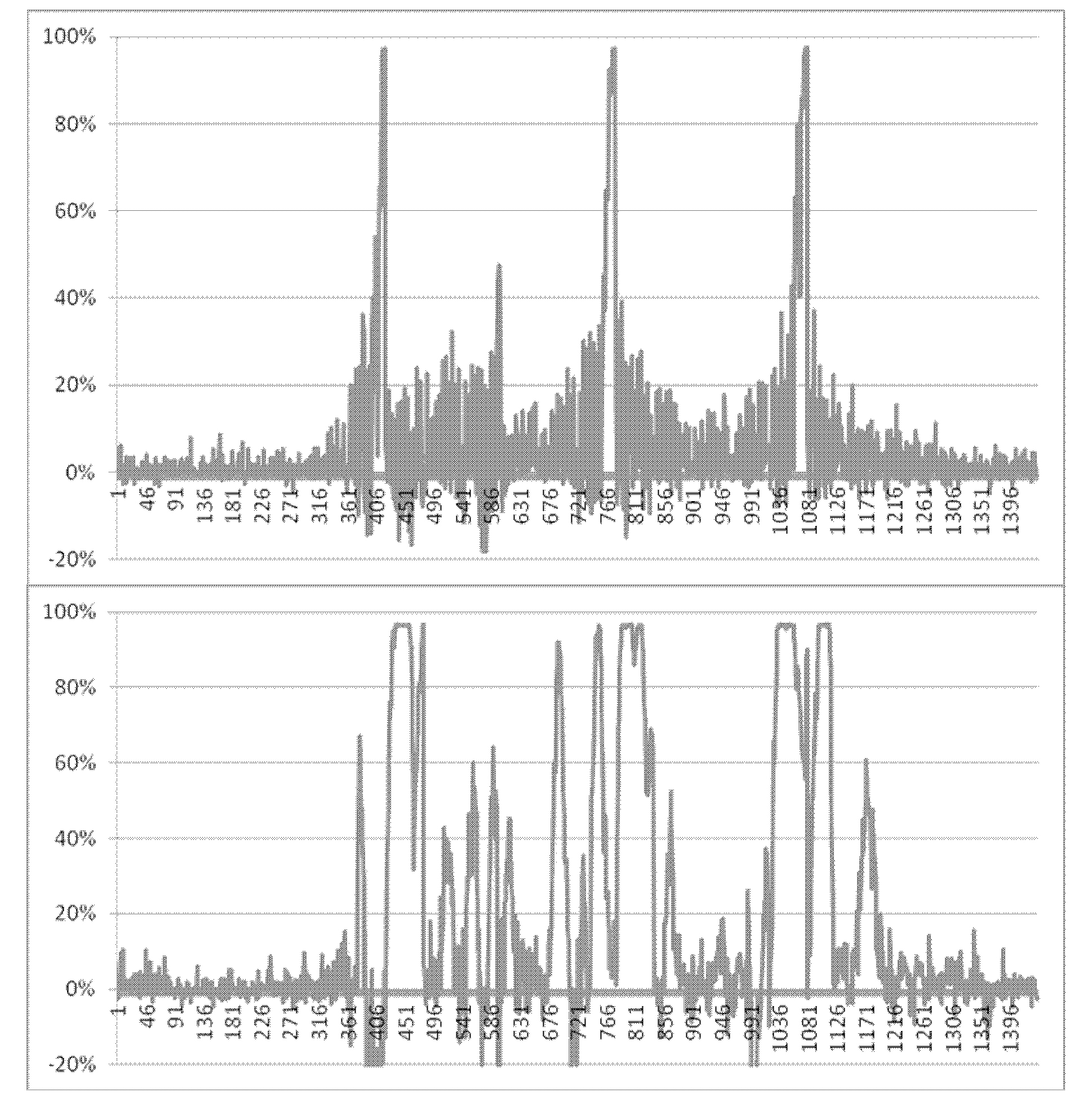
Figure 3.- Reduction of speed in segments of highway
Results
In the base year 2005, a number of 2.3 million vehicle trips are simulated, which includes autos, taxis, and trucks. The main peak hours are at 7am (11 percent of demand), 8am (7 percent), 13 hours (8 percent) and 18 hours (7 percent). For the projected year 2025, a number of 4.2 million vehicle trips are forecasted. The primary performance indicators are presented in Table 2. The comparisons are made from each case to the no-transit case. For the base year 2005, the transit flows in common traffic cause to increase the number of vehicle-hours in between +11 and +18 percent. Also, transit causes to decrease the number of vehicle-miles in between -3 and -5 percent. Therefore, transit reduces speed in between -12 and -20 percent. For the projected year 2025, transit increases the number of vehicle-hours in between +12 and +21 percent, decreases the number of vehicle-miles in between -6 and -10 percent, and decreases speed in between -16 and -25 percent. As a result, transit causes a moderate decrement in the performance of the transportation network. This moderate result can be attributed to the flexibility of the private transportation network, able to use a great number of arterials. Also, this moderate result can be caused by the small capacity and low speed road network of the city of Lima, and as such, capacity reductions will have a small result in an already slow transportation network. The secondary performance indicators are presented in Table 3. For the base year 2005, the transit flows in common traffic increase the user time cost in between +9 and +11 percent. Moreover, the transit flows cause uncertain changes in the user monetary cost ranging between -4 percent and +1 percent. For the projected year 2025, the transit flows increase the user time cost in between +11 and +12 percent, but causes uncertain changes in the user monetary cost in between -5 and +4 percent. However, the net sum of both costs results in a small decrement of the performance of the network in the order of +2 to +4 percent higher cost in 2005 and +3 to +8 percent higher cost in 2025. Consequently, the total of transit flows causes a small decrement in the performance of the entire transportation network in the user time cost and the user monetary cost. The additional performance indicators are also presented in Table 3. For the base year 2005, the transit flows in common traffic worsens the inefficiency factor in between +15 to +24 percent. The transit flows increase the average OD travel time in +3 to +6 percent. Finally, transit flows produce uncertain changes on the daily toll revenues in between +1 and +7 percent. For the projected year 2025, the transit flows increase the inefficiency factor in between +12 and +22 percent, cause uncertain changes of the OD travel time in between -5 and +4 percent, as well as on the daily toll revenues in between 0 and +16 percent. The results of the additional performance indicators confirm that the transit flows causes small decrements in the cost and in the average OD travel time of the entire transportation network, it also causes a moderate increment in the inefficiency factor up to 24 percent, and uncertain changes in the daily revenue tolls. The results on fuel consumption are presented in Table 4. Transit flows cause uncertain changes in fuel consumption. Changes range in the order of between -4 and +2 percent in 2005, and between -6 and +5 percent in 2025. Reason for such uncertain result can be attributed to the flexibility of private transportation in the use of alternative paths, which can be slower or longer. The result on emission of pm10 is presented in Table 4. Transit flows cause uncertain changes in the emission of the pollutant pm10, the changes range from -5 to +2 percent in all estimations. The Figure 2 presents the reduction in productivity speed (mph) by the time of the day, for the case “lane-transit”. In the year 2005, transit flows cause a loss of more than 25 percent in productivity during three hours from 8am to 6pm. In the year 2025, transit flows cause a loss of more than 25 but less of 30 percent in productivity during fourteen hours from 7am to 8pm. In this case, the reduction of productivity by the hour is serious during few hours of 2005 and during most of the hours of 2025. Four individual facilities were analysed in relation to speed by the minute. Each facility was composed of several segments with a total of 18 segments analysed in both directions. As a result of the analysis, most of the segments did not present changes of speed, a few of the segments presented counterintuitive results of increases of speed, and four exceptions presented the expected reduction of productivity. All the exceptions belong to the Central Highway East-West facility which is where the new BRT project is planned, and those exceptions belong to the case “cap-brt-transit”. The segments are located at the West of the Center of the city, where there are more alternative roads for private transportation, but where the intensity of the use of the autos and taxis is much higher than at the East, which is a highway to the mountains of the Andes. The reduction of speed caused by transit reaches an average of +6 percent in 2005 and in +9 percent in 2025, so in average it is a small reduction of speed. However, the reduction of speed grows to serious reductions of speed for certain hours of the day, ranging from +31 percent at 6pm in 2005 to +75 percent at 2pm in 2025. Furthermore, the reduction of speeds reaches very serious reductions of speed for some minutes that correspond to a saturation state, as seen in the Figure 3. In the year 2005, speed reduction can reach +95 percent during some minutes in three occasions that coincide with the peak hours of 7am, 1pm, and 6pm, but most of the time, the reduction of speed is of less than 20 percent. In the year 2025, these periods of very serious reductions of speed or saturation state are extended for more frequent and longer periods of less than 25 minutes, but again, most of the day, the reduction of speed is of less than 20 percent
Conclusions
Transit flows in common traffic have been regarded as a major cause of congestion in developing cities. This paper measures the effect of the transit flows over the performance of an urban transportation network as well as over related variables. As a result, transit flows affect the performance of the transportation network in that: i) Transit flows caused a moderate decrement of speed in -12 to -20 percent in 2005, and of -16 to -25 percent in 2025, ii) Transit flows caused a small increment in user costs and in monetary costs in +2 to +5 percent in 2005 and +3 to +8 percent in 2025, iii) The inefficiency factor can reach moderate increases in the order of +15 to +24 percent in 2005 and in the order of +12 to +22 percent in 2025, iv) Transit flows caused uncertain changes in fuel consumption, in between -4 to +2 percent in 2005 and in between -6 to +5 percent in 2025, v) Transit flows causes uncertain changes in the emission of the pollutant pm10, in between -5 to +2 percent, vi) Transit flows can cause serious reductions of the average speed of the transportation network in the order of more than 25 but less than 30 percent for several hours of the day, vii) In exceptional cases, road facilities can experience very serious reductions of speed in the order of more than 95 percent for some minutes during peak hours in 2005 and for more frequent and longer periods of less than 15 minutes in 2025. But even in those critical cases, the reduction of speed is of less than 20 percent most of the day, viii) As a result, it can be said that, the reduction of the number of transit vehicles as a policy to reduce congestion is not an effective policy due to its small to moderate effects on the transportation network. Also, it is recommended to try other more effective policies with higher priority that can be of and more suitability to individual cases related to the physical characteristics of some road facilities and during certain hours of the day.
Agradecimientos
Funds from CONCYTEC, the Peruvian Council for Science and Technology, made possible the purchase of software and acquisition of data for this research (contract 194-2005-CONCYTEC-OAJ).
References
| [1] | MTC. The Master Plan for Lima and Callao Metropolitan Area Urban Transportation in the Republic of Peru. 2005. |
| [2] | Jacobs, G.D., Fouracre, P.R., and D.A.C. Maunder. “Public Transport in Third World Cities”. The Journal of The Institution of Highway Engineers. March 1982. |
| [3] | Armstrong-Wright, Alan, and Sebastien Thiriez. Bus Services. Reducing Costs, Raising Standards. The World Bank, 1987. |
| [4] | Gwilliam, K., and R. Scurfield. Competition in Public Road Passenger Transport. Paper TWU-39. The World Bank, 1996. |
| [5] | Estache, Antonio, and Andres Gomez-Lobo. The Limits of Competition in Urban Bus Services in Developing Countries. World Bank Policy Research Working Paper 3207. 2004 |
| [6] | Gardner, G., P.R. Cornwell, and J.A. Cracknell. The Performance of Busway Transit in Developing Cities. Research Report 329. TRRL, 1991 |
| [7] | Ardila, Arturo, and Daniel A. Rodriguez. “How Chaos Does Not Destroy Ridership. Operations of an Exclusive Busway Carrying More than 35,000 Passengers per Hour per Direction”. TRR 1726 (2000):1-7. |
| [8] | Diaz, R.B., and Donald C. Schneck. “Bus Rapid Transit Technologies in the Americas. An Overview”. TRR 1731 (2000): 3-9 |
| [9] | Hook, Walter. “Institutional and Regulatory Options for Bus Rapid Transit in Developing Countries. Lessons from International Experience”. TRR 1939 (2005): 184-191 |
| [10] | Tapia, J., and C. Zegrass. “Transporte y Cambio Climatico: Resultados del Estudio de Opciones de Mitigacion” [in Spanish language]. Transporte Urbano y Ambiente, ed. by CONAM (1998:91-96) |
| [11] | MTC. Vitrina, Asistencia Tecnica en Estudios de Transporte Urbano para el Area Metropolitana de Lima y Callao. Informe Final. Informe de Resultados. [in Spanish language] Funded by the World Bank, 1999. |
| [12] | MML. ProTransporte. Estudio de los Impactos Ambientales en el Area de Influencia Directa del Corredor Segregado de Alta Capacidad COSAC / PTUL. [in Spanish language] Preparado por Getinsa / Taryet. Funded by the IAD. 2002 |
| [13] | US-DOT-FHWA. Development and Testing of Dynamic Traffic Assignment and Simulation Procedures for ATIS/ATMS Applications. 1994 |
| [14] | US-DOT-FHWA. Dynasmart-P User´s Guide. 2007. |
| [15] | Pignataro, L.J. Traffic Engineering Theory and Practice. Prentice Hall, 1973. |
| [16] | Douglas, Hummer, and Nelson eds. Manual of Transportation Engineering Studies. 1994 |
| [17] | Martinez, M.J., and J. Cornejo. “Value of the Facilities and Attributes of New Heavy Rail and Bus Rapid Transit Projects in a Developing City. The Case of Lima, Peru”. TRR 1835 (2003): 50-58 |
| [18] | MML. ProTransporte. Perfil de Proyecto Construccion Corredor vial de Transporte Publico Masivo Este-Oeste Carretera Central – Av. Grau – Av. Venezuela, Provincia de Lima. [in Spanish language], 2011 |
E-mail: mjmartinez@pucp.edu.pe
Después borre las líneas borde y vuelva a cuadrar el
Artículo.